Supervised Learning
More information
Here is great tutorial for approaches in machine learning: https://lgatto.github.io/IntroMachineLearningWithR/supervised-learning.html
This covers these topics:
- Introduction
- Preview
- Model performance
- Cross-validation
- Classification performance
- Confusion matrix
- Random forest
- Decision tree
- Data preprocessing
- Missing values
- RSME
- Median imputation
Decision Trees
Decision trees are a method for predicting an outcome from a set of variables. They are great for creating easily-understandable trees.
Class Example
This creates a decision tree to predict a textual (class) output.
library(tidyverse)
library(rpart)
library(rpart.plot)

# Load data into a tibble
t <- tibble(
  temp = c(67, 68, 70, 70, 76, 80, 85, 84, 89, 90, 91, 95, 100),
  raining = c('n', 'n', 'n', 'n', 'n','n','n','n','n','n','y', 'n', 'n'),
  camped = c('Camped', 'No', 'No', 'No', 'No', 'No', 'Camped', 'Camped', 'Camped', 'Camped', 'No', 'No', 'No')
)

# Create the model
# https://stat.ethz.ch/R-manual/R-devel/library/rpart/html/rpart.control.html
#   formula: set output to the Species, and choose input fields
#   data: set to our tibble
#   minsplit: the minimum number of observations that must exist in a node in order for a split to be attempted.
#   minbucket: the minimum number of observations in any terminal
#   method: class, meaning we are predicting a discrete variable
#
m <- rpart(formula = camped ~ temp + raining,
           data = t,
           minsplit = 8,
           minbucket = 5,
           method = "class")

# Show results of model
rpart.plot(m)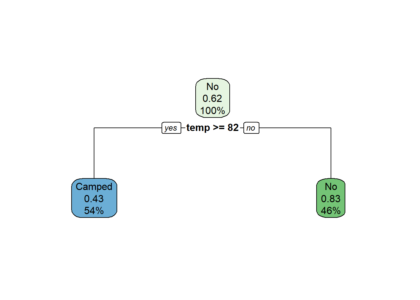
# Create the predicted value and add it to our tibble
predicted <- predict(m, t, type = 'class')
t <- mutate( t,
             predicted = predicted,
             is_correct = predicted == camped)

# Percentage correct
print(mean(t$is_correct))
## [1] 0.6923077# Show a confusion matrix
# Predicted values are in upper case.
table(str_to_upper(t$predicted), t$camped)##
## Camped No
## CAMPED 4 3
## NO 1 5Regression Example
This creates a decision tree to predict a numeric output with regression.
library(tidyverse)
library(rpart)
library(rpart.plot)

# Load data into a tibble
t <- tibble(
  temp = c(67, 68, 70, 70, 76, 80, 85, 84, 89, 90, 91, 95, 100),
  raining = c('n', 'n', 'n', 'n', 'n','n','n','n','n','n','y', 'n', 'n'),
  camped = c('Camped', 'No', 'No', 'No', 'No', 'No', 'Camped', 'Camped', 'Camped', 'Camped', 'No', 'No', 'No')
)

# Create the model
# https://stat.ethz.ch/R-manual/R-devel/library/rpart/html/rpart.control.html
#   formula: set output to the Species, and choose input fields
#   data: set to our tibble
#   minsplit: the minimum number of observations that must exist in a node in order for a split to be attempted.
#   minbucket: the minimum number of observations in any terminal
#   method: class, meaning we are predicting a discrete variable
m <- rpart(formula = temp ~ camped + raining,
           data = t,
           minsplit = 1,
           minbucket = 1,
           method = 'anova')

# Show results of model
rpart.plot(m)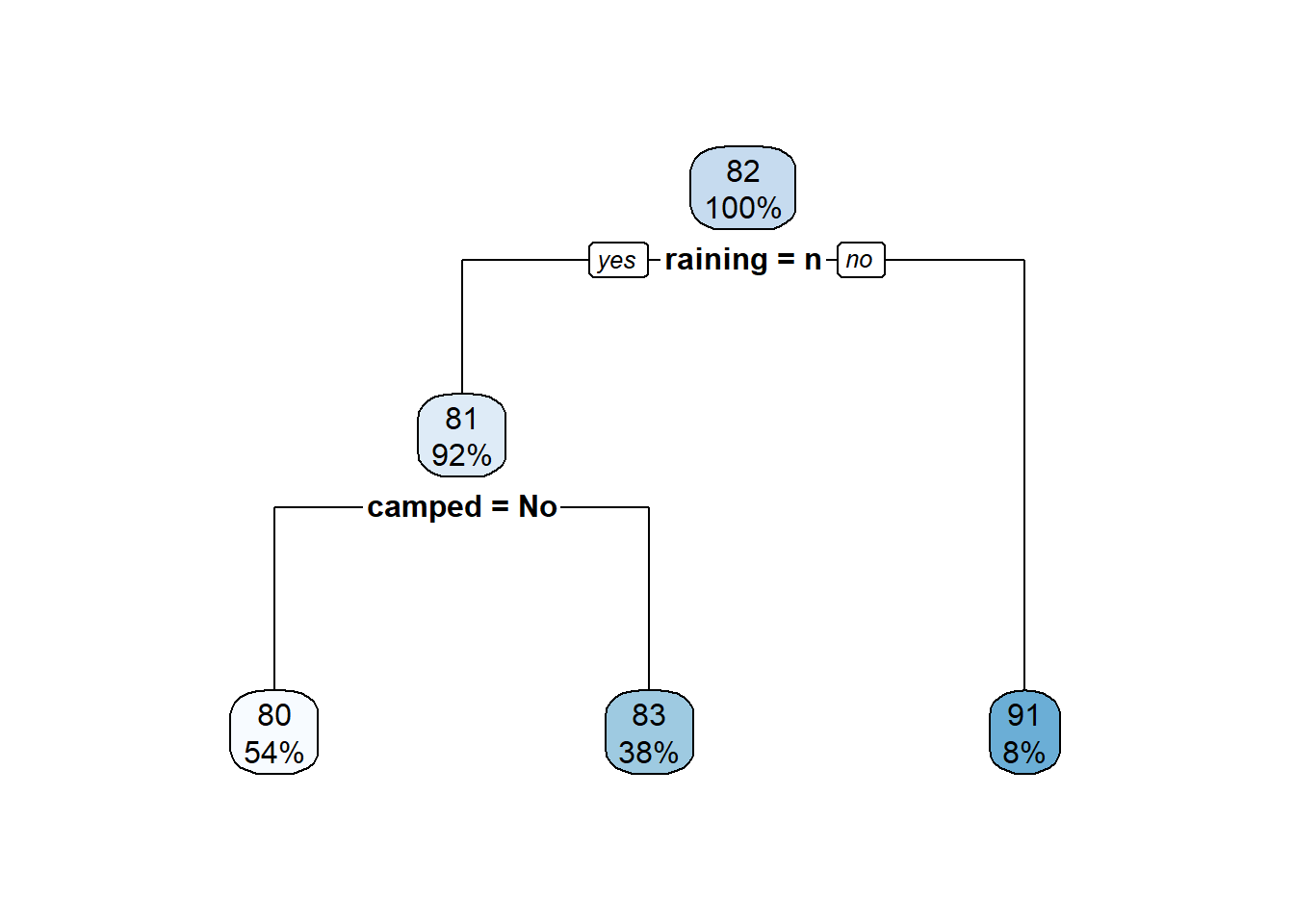
# Create the predicted value and add it to our tibble
predicted <- predict(m, t)
t <- mutate( t,
             predicted = predicted,
             residual = predicted - temp)

# Residual value
hist(t$residual)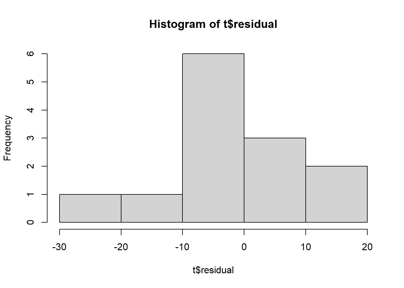
Random Forest
A random forest is an upgraded decision tree. It creates a very large number of decision trees, and then combines them to build a more accurate model. One of the key benefits is that it can handle a large number of variables.
Sampling in a random forest works differently than in a decision tree. In a decision tree, we use the entire dataset (or split it between training and testing datasets). In a random forest, each tree uses a random sample of the data. Then, at each decision point, it uses a random subset of the columns. This helps to prevent overfitting.
Help:
Class Example
This creates a decision tree to predict a textual (class) output. Our key outcome is the oob misclassification rate (out of bag). We use all of the data except one to train the model, and then use that one item to test the model. This is repeated multiple times.
library(tidyverse)
library(randomForestSRC)


# Load data into a tibble
t <- tibble(
  temp = c(67, 68, 70, 70, 76, 80, 85, 84, 89, 90, 91, 95, 100),
  raining = c(0, 0, 1, 1, 1, 0, 0, 0, 1, 1, 1, 0, 0),
  camped_as_text = c('Camped', 'No', 'No', 'No', 'No', 'No', 'Camped', 'Camped', 'Camped', 'Camped', 'No', 'No', 'No')
)

# We must set all text variables (class) as factors.
t <- t %>%
  mutate(camped_as_factor = as.factor(camped_as_text),
         camped_as_text = NULL)

# Set the random number generator so we have consistent results.
set.seed(1)

# Note that we *must* convert from a tibble into a dataframe.
#   ntree: number of trees
#   mtry: number of variables to try at each node (default is 3 for regression, or sqrt(variables))
#   nodesize: the number of items at each ending node. Defaults to 5 for regression and 1 for classification.
#   na.action: what to do with missing values, either 'na.omit' (default) or 'na.impute'
rf_model <- rfsrc(camped_as_factor ~ .,
                  data = as.data.frame(t),
                  ntree = 500)

# Measure our accuracy according to the oob misclassification rate (out of bag) .
# This is the % of times that our model got the wrong prediction.
print(rf_model)
## Sample size: 13
## Frequency of class labels: 5, 8
## Number of trees: 500
## Forest terminal node size: 1
## Average no. of terminal nodes: 3.566
## No. of variables tried at each split: 2
## Total no. of variables: 2
## Resampling used to grow trees: swor
## Resample size used to grow trees: 8
## Analysis: RF-C
## Family: class
## Splitting rule: gini *random*
## Number of random split points: 10
## Imbalanced ratio: 1.6
## (OOB) Brier score: 0.24999205
## (OOB) Normalized Brier score: 0.99996819
## (OOB) AUC: 0.575
## (OOB) Log-loss: 0.88115792
## (OOB) PR-AUC: 0.46824018
## (OOB) G-mean: 0.72456884
## (OOB) Requested performance error: 0.23076923, 0.4, 0.125
##
## Confusion matrix:
##
## predicted
## observed Camped No class.error
## Camped 3 2 0.400
## No 1 7 0.125
##
## (OOB) Misclassification rate: 0.2307692# Look at the variable importance, basically the most important variables in our dataset.
#
# vimp works by comparing the accuracy of a model with the variable and without it.
# The difference is the importance of the variable.
vimp_results <- vimp(rf_model, importance = TRUE)$importance
print(round(vimp_results, 2))## all Camped No
## temp 0.16 0.36 0.46
## raining 0.00 -0.03 0.00Regression Example
This creates a decision tree to predict a number output. Our key outcome is the oob misclassification rate (out of bag). We use all of the data except one to train the model, and then use that one item to test the model. This is repeated multiple times.
library(tidyverse)
library(randomForestSRC)


# Load data into a tibble
t <- tribble(
  ~temp, ~water, ~fog, ~snow,
  'freezing', 1.2, 'y', 2.3,
  'freezing', 0.2, 'y', .4,
  'freezing', 1.2, 'y', .4,
  'freezing', 0, 'y', 0,
  'freezing', 0, 'y', 0,
  'freezing', 0, 'y', 0,
  'freezing', 0, 'y', 0,
  'freezing', 1.5, 'n', 2,
  'freezing', 0, 'y', 0,
  'hot', 0, 'n', 0,
  'hot', 0, 'n', 0,
  'hot', 0, 'n', 0,
  'hot', 1.5, 'n', 0,
  'hot', 1.5, 'n', 0,
  'hot', 1.5, 'n', 0,
  'hot', 1.5, 'n', 0,
  'hot', 1.2, 'n', 0,
  'hot', 0, 'y', 0
)

# We must set all text variables (class) as factors.
t <- t %>%
  mutate(fog_as_factor = as.factor(fog),
         fog = NULL,
         temp_as_factor = as.factor(temp),
         temp = NULL)

# Set the random number generator so we have consistent results.
set.seed(1)

# Note that we *must* convert from a tibble into a dataframe.
#   ntree: number of trees
#   mtry: number of variables to try at each node (default is 3 for regression, or sqrt(variables))
#   nodesize: the number of items at each ending node. Defaults to 5 for regression and 1 for classification.
#   na.action: what to do with missing values, either 'na.omit' (default) or 'na.impute'
rf_model <- rfsrc(snow ~ .,
                  data = as.data.frame(t),
                  ntree = 500)

# Measure our accuracy according to the oob misclassification rate (out of bag) .
# This is the % of times that our model got the wrong prediction.
print(rf_model)
## Sample size: 18
## Number of trees: 500
## Forest terminal node size: 5
## Average no. of terminal nodes: 1.982
## No. of variables tried at each split: 1
## Total no. of variables: 3
## Resampling used to grow trees: swor
## Resample size used to grow trees: 11
## Analysis: RF-R
## Family: regr
## Splitting rule: mse *random*
## Number of random split points: 10
## (OOB) R squared: 0.02733811
## (OOB) Requested performance error: 0.46716379Neural Network - simple class
Good reference videos:
We will use the NeuralNet library.
Build a model
Below is a simple model created from some sample fraud data. It predicts a simple 0/1 outcome.
library(neuralnet)
library(tidyverse)

t_train <- tribble(
  ~fraud, ~jail01, ~age01, ~grump01,
  1, 1, .5, .5,
  1, 1, 1, 0,
  1, 1, 0, 1,
  1, 0, .75, .8,
  1, 0, .6, 1,
  1, 1, .5, .9,
  0, 0, 0, 1,
  0, 0, 0, 0,
  0, 0, 1, 1,
  0, 0, 1, .8,
  )

t_test <- tribble(
  ~fraud, ~jail01, ~age01, ~grump01,
  1, 1, 0, 0,
  1, 1, .5, .25,
  0, 0, 0, 1,
  0, 0, 0, 0,
  0, 0, .9, .9,
  0, 0, 7, .5,
)


# Set the random number generator's starting value. This makes our outputs repeatable, so we
# don't get different results each time we run our software.
set.seed(1)

# The neuralnet function creates our model.
# Arguments:
#   formula: dependent variable ~ indepedent variables + ...
#   data: our tibble
#   hidden: how many hidden nodes should we use? Use an integer
#   linear.output: generally T for regression or F for classification
n <- neuralnet(fraud ~ jail01 + age01,
               data = t_train,
               hidden = 1,
               linear.output = FALSE)

# View output
# Input notes are on the left, intermediate in the center, and output on the right.
# Steps tells us how many times the algorithm iterated through before stopping
# Error is the sse, but other options are also available.
plot(n)
Measure accuracy on training data
# Continue the previous code block, ...


# Measure accuracy on training set
# This code makes a new tibble showing the results in a easy to grasp form.
#   prediction: this is the output of our model. Use net.result[[1]] to grab the first item returned.
#   prediction01: the prediction outputs a decimal number. Since this problem has a 0/1, round.
prediction = n$net.result[[1]]
prediction01 = round(prediction, digits = 0)

# Create a confusion table
# Prediction is on the left, and actual on the top.
#
#             0                1       <===  Actual outcome
# 0    Negative was True    Negative was False
# 1    Positive was False   Positive was True
# ^
#  \
#    prediction
#
train_table <- table(prediction01, t_train$fraud )
print(train_table)
##
## prediction01 0 1
## 0 2 0
## 1 2 6# Use coordinates to access our truth table
# We start at the top-left corner with [1,1], with [line, column]
#
# 0 1
# 0 [1, 1] [1, 2]
# 1 [2, 1] [2, 2]
# Accuracy: true / total
# What is the total number of cases properly classified?
train_accuracy <- (train_table[1, 1] + train_table[2, 2]) / sum(train_table)
# Recall: true positives / (true positives + false negative)
# How many of the target cases did we find?
train_recall <- train_table[2, 2] / (train_table[1, 2] + train_table[2, 2])
# Precision: true positives / (false positive + true positive)
train_precision <- train_table[2, 2] / (train_table[2, 1] + train_table[2, 2])
print(paste('Accuracy', train_accuracy))## [1] "Accuracy 0.8"print(paste('Recall', train_recall))## [1] "Recall 1"print(paste('Precision', train_precision))## [1] "Precision 0.75"Evaluate on test data
# Continue the previous code block, ...

# Now try test data.
#   n is our model
#   t_test is our data
p <- predict(n, t_test)

# Evaluate the success by looking at the returned vector
# Note that we get a matrix back. We just want a vector, so access
# by using [ , 1] <--- return all rows, but only first column.
prediction = p[,1]
prediction01 = round(prediction, digits = 0)

confusion <- table(prediction01, t_test$fraud)

print(confusion)
##
## prediction01 0 1
## 0 2 0
## 1 2 2Neural Network - multiple classes
Build a model
We can use textual data. It will be encoded with each value set to a 0 or 1 field.
library(neuralnet)
library(tidyverse)

# Load our iris dataset
data(iris)

set.seed(1)

# Create a sample vector of 1 and 0s, with 70% 1st and 30% 0.
index <- sample( c(1, 0),
                 nrow(iris),
                 replace = TRUE,
                 prob = c(.7, .3) )

# Split data into test/train
t_train <- filter( iris, index == 1 )
t_test <- filter( iris, index == 0)

# Train algorithm
# Note that we are using a textual output, so instead of a single output node
# we now have one per label.
#   linear.output: generally T for regression or F for classification
n <- neuralnet(Species  ~ Sepal.Length + Sepal.Width + Petal.Length + Petal.Width,
               data = t_train,
               hidden = 2,
               linear.output = FALSE)

plot(n)
Measure accuracy on training data
Below is some sample code to measure the accuracy of the training / test data.
# continue previous...

# Grab the matrix of results and round to the 0
matrix = round(n$net.result[[1]], digits = 0)

# Add column names
colnames(matrix) <- list('setosa_node', 'versicolor_node', 'virginica_node')

# Convert matrix to a tibble
#     Add a column called predicted that says if we are
#     predicting setota, versicolor, or virginica.
t_results <- as.tibble(matrix)  %>%
  mutate(predicted = ifelse(setosa_node == 1, 'setosa',
                            ifelse(versicolor_node == 1, 'versicolor', 'virginica')))


# Test accuracy with original data
accuracy = mean(t_results$predicted == t_train$Species)
print(accuracy)
## [1] 0.990566# See confusion table
table(str_to_upper(t_results$predicted), t_train$Species)##
## setosa versicolor virginica
## SETOSA 34 0 0
## VERSICOLOR 0 34 1
## VIRGINICA 0 0 37Measure accuracy on test data
Below is some sample code to measure the accuracy of the training / test data.
# continue previous...

predictions <- predict(n, t_test)

# Grab the matrix of results and round to the 0
matrix = round(predictions, digits = 0)

# Add column names
colnames(matrix) <- list('setosa_node', 'versicolor_node', 'virginica_node')

# Convert to tibble
t_results <- as.tibble(matrix)  %>%
  mutate(predicted = ifelse(setosa_node == 1, 'setosa',
                            ifelse(versicolor_node == 1, 'versicolor', 'virginica')))


# Test accuracy with original data
accuracy = mean(t_results$predicted == t_test$Species)
print(accuracy)
## [1] 0.9318182# See confusion table
table(t_results$predicted, t_test$Species)##
## setosa versicolor virginica
## setosa 16 1 0
## versicolor 0 15 2
## virginica 0 0 10Neural Network - numeric output
Build a model
Below is a simple model predicting a numerical outcome. We use the mtcars dataset.
library(neuralnet)
library(tidyverse)

t <- tribble(
  ~height, ~weight, ~is_sumo,
  100, 100, 1,
  200, 190, 0,
  150, 130, 1,
  80, 200, 0,
  175, 200, 1,
  100, 80, 1,
  90, 70, 1,
  210, 200, 1,
  150, 160, 0,
  110, 140, 0,
  175, 200, 1,
  103, 80, 1
)

# Scale the data and add a 0/1
is_test = sample(x = c(0, 1),
                 size = 12,
                 replace = TRUE,
                 prob = c(0.5, 0.5))

# Setup the data to be scaled and have a 1/0 test/train variable
t <- t %>%
  mutate(is_test = is_test,
         height = scale(height),
         weight = scale(weight))


# Setup train/test tibbles
t_train <- filter(t, is_test == 0)
t_test <- filter(t, is_test == 1)


# Set the random number generator's starting value. This makes our outputs repeatable, so we
# don't get different results each time we run our software.
set.seed(1)

# The neuralnet function creates our model.
# Arguments:
#   formula: dependent variable ~ indepedent variables + ...
#   data: our tibble
#   hidden: how many hidden nodes should we use? Use an integer
#   linear.output: generally T for regression or F for classification
n <- neuralnet(formula = height ~ weight + is_sumo,
               data = t_train,
               hidden = 1,
               linear.output = TRUE)

# View output
# Input notes are on the left, intermediate in the center, and output on the right.
# Steps tells us how many times the algorithm iterated through before stopping
# Error is the sse, but other options are also available.
plot(n)
Measure accuracy on training data
# Continue the previous code block, ...


# Measure accuracy on training set
# This code makes a new tibble showing the results in a easy to grasp form.
#   prediction: this is the output of our model. Use net.result[[1]] to grab the first item returned.
prediction = n$net.result[[1]]

# Show error in a nice format
t_train <- t_train %>%
  mutate(prediction = prediction,
         residual = prediction - weight)

# Show predicted v. actual
print(t_train)
## # A tibble: 7 × 6
## height[,1] weight[,1] is_sumo is_test prediction[,1] residual[,1]
## <dbl> <dbl> <dbl> <dbl> <dbl> <dbl>
## 1 -0.814 -0.868 1 0 -0.722 0.146
## 2 1.39 0.836 0 0 1.41 0.570
## 3 0.289 -0.300 1 0 0.258 0.558
## 4 -0.814 -1.25 1 0 -0.836 0.410
## 5 1.61 1.03 1 0 1.61 0.580
## 6 -0.594 -0.110 0 0 -0.561 -0.451
## 7 -0.748 -1.25 1 0 -0.836 0.410# Find the sse
print((sum(t_train$residual ^ 2)))## [1] 1.533005Evaluate on test data
# Continue the previous code block, ...

# Now try test data.
#   n is our model
#   t_test is our data
p <- predict(n, t_test)

# Evaluate the success by looking at the returned vector
# Note that we get a matrix back. We just want a vector, so access
# by using [ , 1] <--- return all rows, but only first column.
prediction = p[,1]

# Show error in a nice format
t_test <- t_test %>%
  mutate(prediction = prediction,
         residual = prediction - weight)

# Show predicted v. actual
print(t_test)
## # A tibble: 5 × 6
## height[,1] weight[,1] is_sumo is_test prediction residual[,1]
## <dbl> <dbl> <dbl> <dbl> <dbl> <dbl>
## 1 -1.26 1.03 0 1 1.52 0.496
## 2 0.840 1.03 1 1 1.61 0.580
## 3 -1.03 -1.44 1 1 -0.851 0.585
## 4 0.289 0.268 0 1 0.235 -0.0332
## 5 0.840 1.03 1 1 1.61 0.580# Find the the sse
print((sum(t_test$residual ^ 2)))## [1] 1.261366Scaling data
Scale is a useful function for rescaling a set of input data.
# Rescale data
#   x: vector of data input
#   center: boolean, do we subtract column mean from each value (so mean = 0)?
#   scale: boolean, do we divide data by the sd after centering?
x2 <- scale(x = c(1, 2, 3, 4, 4, 5,3),
      center = TRUE,
      scale = TRUE)

summary(x2)
## V1
## Min. :-1.5930
## 1st Qu.:-0.4779
## Median :-0.1062
## Mean : 0.0000
## 3rd Qu.: 0.6372
## Max. : 1.3806# We can also use the short form of this, relying on the defaults to get the
# same result as above.
summary(scale(c(1, 2, 3, 4, 4, 5,3)))## V1
## Min. :-1.5930
## 1st Qu.:-0.4779
## Median :-0.1062
## Mean : 0.0000
## 3rd Qu.: 0.6372
## Max. : 1.3806# We will often need to rescale the output to get it back into the normal form.
# attributes:
# dim
# scaled:center
# scaled:scale
attributes(x2)## $dim
## [1] 7 1
##
## $`scaled:center`
## [1] 3.142857
##
## $`scaled:scale`
## [1] 1.345185# Get only the new data
scaled_data <- x2[,1]
print(scaled_data)## [1] -1.5929827 -0.8495908 -0.1061988 0.6371931 0.6371931 1.3805850 -0.1061988# Rescale by multiplying by the scale and adding the center.
scaled_data * attr(x2, 'scaled:scale') + attr(x2, 'scaled:center')## [1] 1 2 3 4 4 5 3