course_model

Principle Component Analysis (PCA)

PCA is a method for reducing the number of columns while retaining as much information as possible.

Outcomes

Understand the PCA algorithm
Apply PCA for dimensionality reduction

PCA Algorithm

Principal Component Analysis (PCA) is a technique for:

Reducing dimensionality (many features → fewer features),
While preserving as much variance as possible,
By creating new, uncorrelated features called principal components.

Each principal component is:

A linear combination of the original features.
Orthogonal (perpendicular) to the others.
Ordered so that:
- PC1 explains the most variance,
- PC2 explains the second most variance,
- etc.

import numpy as np
import pandas as pd
from sklearn.preprocessing import StandardScaler
from sklearn.decomposition import PCA

# Create a dataset
df = pd.DataFrame({
    'height': [10, 12, 13, 15, 18, 20, 22, 25, 30, 35, 40, 45, 50, 55, 60, 65, 70],
    'weight': [30, 32, 35, 40, 45, 50, 55, 60, 65, 70, 75, 80, 85, 90, 95, 100, 105],
    'age': np.random.randint(20, 60, size=17)
})

# PCA works best when features are centered; standardization is often used when units differ.
X = df[['height', 'weight', 'age']].values  # shape: (17, 3)
scaler = StandardScaler()
X_scaled = scaler.fit_transform(X) 
# `X_scaled` has mean ~0 and variance ~1 in each column.

# Fit PCA
pca = PCA(n_components=2)
X_pca = pca.fit_transform(X_scaled)

# `pca.components_` is a 2×3 matrix. Each row is a principal component (PC1 and PC2), each column corresponds to a feature (`height`, `weight`, `age`).
# `pca.explained_variance_ratio_` might look something like `[0.95, 0.05]`, meaning the amount of variance captured by each principal component.
print("Principal components (directions):")
print(pca.components_)

print("\nExplained variance ratio:")
print(pca.explained_variance_ratio_)

Principal components (directions):
[[ 0.70317421  0.70333577 -0.10423451]
 [ 0.07527239  0.07213746  0.99455028]]

Explained variance ratio:
[0.66635142 0.32967702]

Add PCA results back to a DataFrame

We can now use the PCA results to do further analysis or visualization.

df_pca = pd.DataFrame(
    X_pca,
    columns=['PC1', 'PC2']
)

df_with_pca = pd.concat([df.reset_index(drop=True), df_pca], axis=1)

import matplotlib.pyplot as plt

# Plot PCA-transformed data with two scatter calls (matplotlib scatter marker must be a single style)
plt.figure(figsize=(12, 5))

young = df_with_pca[df_with_pca['age'] < 30]
middle = df_with_pca[(df_with_pca['age'] >= 30) & (df_with_pca['age'] < 45)]
old = df_with_pca[df_with_pca['age'] >= 45]

plt.scatter(
    young['PC1'], young['PC2'],
    c=young['height'] + young['weight'],
    marker='.', cmap='viridis', alpha=0.7, label='age < 30'
)
plt.scatter(
    middle['PC1'], middle['PC2'],
    c=middle['height'] + middle['weight'],
    marker='*', cmap='viridis', alpha=0.7, label='30 ≤ age < 45'
)
plt.scatter(
    old['PC1'], old['PC2'],
    c=old['height'] + old['weight'],
    marker='o', cmap='viridis', alpha=0.7, label='age ≥ 45'
)

plt.colorbar(label='height + weight')
plt.xlabel('PC1')
plt.ylabel('PC2')
plt.title('PCA Scatter (Age-Based Markers)')
plt.legend()
plt.tight_layout()
plt.show()

png

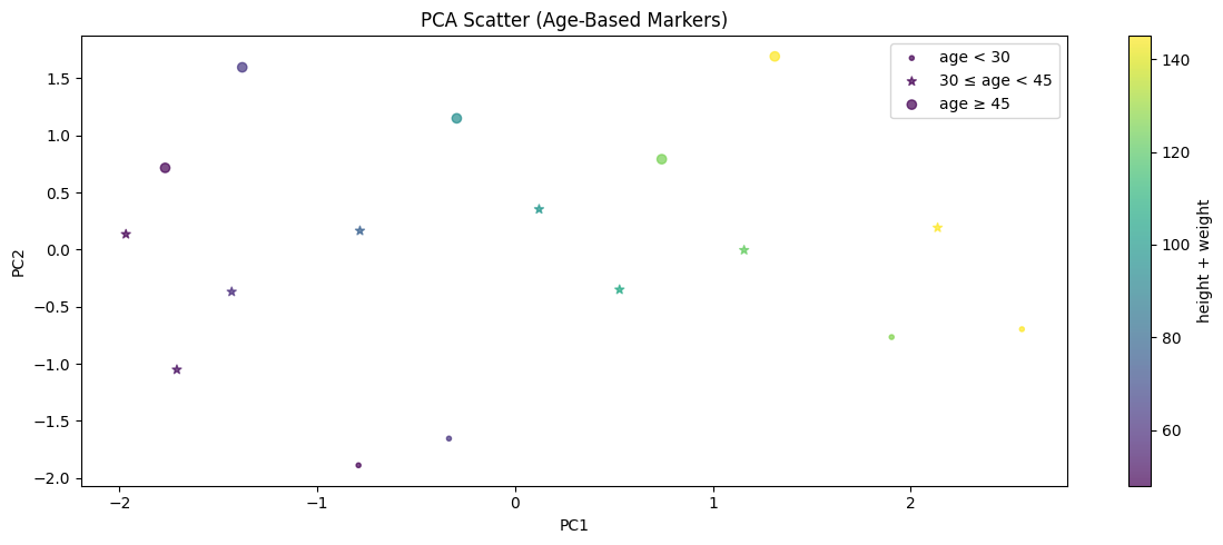
Example PCA Process

This image show the PCA training process on a dataset with three features reduced to two principal components. PCA Process