course_model

Principle Component Analysis (PCA)

PCA is a method for reducing the number of columns while retaining as much information as possible.

Outcomes:

Explain the basics of the PCA algorithm
Define variance, principal components, and orthogonal
Explain why we want to reduce the number of columns in a dataset
Explain why we may add the PCs back onto an original dataset
Explain how graphing the PCs can help us understand the data
Apply PCA for dimensionality reduction

Links

template census data and PCA example

PCA Algorithm

Principal Component Analysis (PCA) is a technique for:

Reducing dimensionality (many features → fewer features),
While preserving as much variance as possible,
By creating new, uncorrelated features called principal components.

Each principal component is:

A linear combination of the original features.
Orthogonal (perpendicular) to the others.
Ordered so that:
- PC1 explains the most variance,
- PC2 explains the second most variance,
- etc.

import numpy as np
import pandas as pd
from sklearn.preprocessing import StandardScaler
from sklearn.decomposition import PCA

# Create a dataset of predefined car samples
df = pd.DataFrame({
    'engine_displacement': [1.5, 2.0, 2.5, 3.0, 3.5, 4.0, 4.5, 5.0, 5.5, 6.0, 6.5, 7.0, 7.5, 8.0, 1.8, 2.2, 2.8, 3.5, 4.2, 5.5],
    'num_cylinders': [3, 4, 4, 4, 5, 6, 6, 8, 8, 8, 10, 10, 12, 12, 4, 4, 6, 6, 8, 8],
    'engine_power': [120, 160, 200, 250, 280, 320, 380, 450, 520, 580, 600, 640, 650, 720, 140, 180, 300, 350, 520, 600],
    'price': [25000, 32000, 38000, 45000, 52000, 60000, 72000, 85000, 95000, 110000, 125000, 135000, 145000, 150000, 28000, 35000, 55000, 65000, 90000, 120000],
    'weight': [2500, 2700, 2900, 3100, 3300, 3600, 3900, 4200, 4500, 4700, 4900, 5000, 5100, 5200, 2600, 2800, 3200, 3500, 4300, 4600],
    'mpg': [38, 32, 28, 25, 22, 20, 18, 16, 14, 12, 11, 10, 9, 8, 35, 30, 21, 19, 15, 12],
    'year': [2023, 2023, 2023, 2022, 2022, 2022, 2021, 2021, 2020, 2020, 2019, 2019, 2018, 2018, 2023, 2023, 2022, 2022, 2021, 2020],
    'acceleration': [10.5, 8.2, 7.1, 6.5, 6.0, 5.5, 5.0, 4.5, 4.2, 3.9, 3.7, 3.5, 3.3, 3.0, 9.8, 8.0, 6.8, 6.2, 4.8, 4.0]
})

# Add car type classification
df['car_type'] = df.apply(
    lambda row: 'Sports Car' if (row['engine_power'] >= 400 or row['acceleration'] < 5.0) else 'Economy Car',
    axis=1
)

# PCA works best when features are centered; standardization is often used when units differ.
X = df[['engine_displacement', 'num_cylinders', 'engine_power', 'price', 'weight', 'mpg', 'year', 'acceleration']].values  # shape: (20, 8)
scaler = StandardScaler()
X_scaled = scaler.fit_transform(X) 
# `X_scaled` has mean ~0 and variance ~1 in each column.

# Fit PCA
pca = PCA(n_components=2)
X_pca = pca.fit_transform(X_scaled)

print("Principal components (directions):")
print(pca.components_)

Principal components (directions):
[[ 0.35663352  0.35106612  0.35776287  0.35699674  0.35874068 -0.35013588
  -0.35279264 -0.34405162]
 [ 0.13807797  0.35411536  0.01102768  0.24256939 -0.01602305  0.49075458
  -0.38000873  0.64114884]]

# Show how the principal component scores map back into the original variables
print("\nPrincipal component scores (projections):")
print(X_pca)

# Display loadings - how each variable aligns with each component
feature_names = ['engine_displacement', 'num_cylinders', 'engine_power', 'price', 'weight', 'mpg', 'year', 'acceleration']
loadings_df = pd.DataFrame(
    pca.components_.T,
    columns=['PC1', 'PC2'],
    index=feature_names
)

print("\n\nLoadings - Alignment of Variables with Principal Components:")
print("(Shows how strongly each variable contributes to each PC)")
print(loadings_df)

print("\n\nVariable Contributions (sorted by absolute value):")
print("\nPC1 - Top contributors:")
print(loadings_df['PC1'].abs().sort_values(ascending=False))
print("\nPC2 - Top contributors:")
print(loadings_df['PC2'].abs().sort_values(ascending=False))

Principal component scores (projections):
[[-4.47305525  1.01239304]
 [-3.41510905  0.18644614]
 [-2.77413926 -0.30144973]
 [-2.01184745 -0.34278791]
 [-1.38674124 -0.45324969]
 [-0.7335913  -0.50296825]
 [ 0.07604103 -0.42887747]
 [ 0.96266473 -0.31329746]
 [ 1.74070809 -0.18980161]
 [ 2.28919508 -0.26651954]
 [ 3.18508469  0.23903071]
 [ 3.55484559  0.2190217 ]
 [ 4.34716719  0.6955037 ]
 [ 4.74551173  0.61650451]
 [-3.94681628  0.80369696]
 [-3.16107063  0.04555603]
 [-1.45018632 -0.16103636]
 [-0.83915274 -0.34751079]
 [ 1.02302003 -0.30238363]
 [ 2.26747136 -0.20827034]]


Loadings - Alignment of Variables with Principal Components:
(Shows how strongly each variable contributes to each PC)
                          PC1       PC2
engine_displacement  0.356634  0.138078
num_cylinders        0.351066  0.354115
engine_power         0.357763  0.011028
price                0.356997  0.242569
weight               0.358741 -0.016023
mpg                 -0.350136  0.490755
year                -0.352793 -0.380009
acceleration        -0.344052  0.641149


Variable Contributions (sorted by absolute value):

PC1 - Top contributors:
weight                 0.358741
engine_power           0.357763
price                  0.356997
engine_displacement    0.356634
year                   0.352793
num_cylinders          0.351066
mpg                    0.350136
acceleration           0.344052
Name: PC1, dtype: float64

PC2 - Top contributors:
acceleration           0.641149
mpg                    0.490755
year                   0.380009
num_cylinders          0.354115
price                  0.242569
engine_displacement    0.138078
weight                 0.016023
engine_power           0.011028
Name: PC2, dtype: float64

Add PCA results back to a DataFrame

We can now use the PCA results to do further analysis or visualization.

df_pca = pd.DataFrame(
    X_pca,
    columns=['PC1', 'PC2']
)

df_with_pca = pd.concat([df.reset_index(drop=True), df_pca], axis=1)

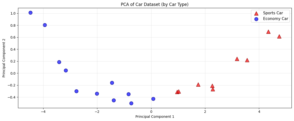
import matplotlib.pyplot as plt

# Plot PCA-transformed data colored and shaped by car type
plt.figure(figsize=(12, 5))

# Separate data by car type
sports_cars = df_with_pca[df_with_pca['car_type'] == 'Sports Car']
economy_cars = df_with_pca[df_with_pca['car_type'] == 'Economy Car']

# Plot each group with different color and marker shape
plt.scatter(sports_cars['PC1'], sports_cars['PC2'], c='red', marker='^', s=120, alpha=0.7, label='Sports Car', edgecolors='darkred', linewidth=1.5)
plt.scatter(economy_cars['PC1'], economy_cars['PC2'], c='blue', marker='o', s=100, alpha=0.7, label='Economy Car', edgecolors='darkblue', linewidth=1.5)

plt.xlabel('Principal Component 1')
plt.ylabel('Principal Component 2')
plt.title('PCA of Car Dataset (by Car Type)')
plt.legend(fontsize=11)
plt.grid(alpha=0.3)
plt.tight_layout()
plt.show()

png

Example PCA Process

This image show the PCA training process on a dataset with three features reduced to two principal components. PCA Process